The OpenBCI GUI is a free program that connects to an OpenBCI board, such as the Cyton, the Cyton with Daisy, or the Ganglion, and turns its raw electrical readings into something you can see, record, clean up and send elsewhere. It is the first thing most people open after unboxing their kit, and for many it is the only tool they need for months.
OpenBCI describes seven reasons people use it. On paper they read like a feature list. In practice, each one solves a real problem that researchers, students, teachers and hobbyists run into. This article takes each use case in turn and answers three questions:
- What it means, in plain language.
- Why it is useful, with real situations where it matters.
- How to do it, with concrete steps and the mistakes to avoid.
It is written for beginners. If you have never recorded EEG, electroencephalography, the measurement of the brain’s electrical activity through the scalp, you can still follow every section. The examples come from a Cyton + Daisy setup with a gel cap, but most apply to any OpenBCI board.
1. Visualizing brainwaves in real time
The GUI’s main job is to show your brain’s electrical activity live, the moment it happens, in several different views at once.
What it means
The screen is split into panels called widgets. Each widget shows the same incoming data in a different way, and you can swap any panel to any widget from the dropdown in its corner. The most useful ones are:

The widget menu, circled in red. This panel currently shows the Time Series; click the name to switch it to any other widget.
| Widget | What it shows | Best for |
| Time Series | Each electrode’s signal as a moving line | Checking electrode quality; spotting blinks and movement |
| FFT Plot | Which rhythms (frequencies) are present and how strong | Spotting the 10 Hz alpha rhythm; finding electrical hum |
| Band Power | The same, summed into five bars: delta, theta, alpha, beta, gamma | Quick, readable summaries for audiences |
| Spectrogram | Rhythms changing over time, as a heat map | Watching alpha rise when eyes close |
| Head Plot | A top-down head coloured by activity | Showing where activity is |
| Accelerometer | The board’s motion sensor | Ruling out movement as the cause of noise |
| EMG | Muscle activity as bars | Jaw clenches, facial movements, arm muscles |
Why it is useful
- Checking signal quality before recording. The Time Series shows at a glance whether each electrode is working. A label reading “Railed” means the amplifier is overloaded, usually from poor contact; “Not Railed” with a small µVrms value, roughly 5 to 50, means the channel is measuring properly. Fixing problems here saves hours of unusable data later.
- Teaching and outreach. Nothing explains EEG faster than letting someone blink and watch a spike appear. Live visuals turn an abstract idea into something people can see.
- Live demos. At an open day or lab demo, the Time Series, EMG and Band Power widgets side by side make changes obvious to a crowd.
- Spotting problems early. A spike at 60 Hz on the FFT plot means power-line hum; a flat line at 0.00 µVrms means nothing is connected.

How to put widgets side by side. First click Layout to choose how many panels the screen shows. Then use each panel’s widget menu to pick what it displays; here, Time Series on the left and FFT Plot on the right.
How to do it
- Click Layout at the top right and choose how many panels you want. Three or four is a good balance.
- Set one panel to Time Series, one to FFT Plot, and one to Band Power or EMG, depending on your purpose.
- In the Time Series, set Vert Scale, which works like a zoom, to 200 µV while you are setting up. That keeps even big, messy signals on screen, so you can see which electrodes need fixing. Once the signals settle down and look small and calm, change it to 100 µV to zoom in, so the real brain activity is easy to see. This only changes the view, not what gets recorded.
- Try the classic test: ask the wearer to close their eyes and relax for 10 seconds. When we relax with our eyes closed, the part of the brain that handles vision, at the back of the head, slips into a steady “idling” wave that repeats about 10 times a second. If you have electrodes at the back of the head (O1 and O2), this shows up on the FFT plot as a clear bump at about 10 Hz, and it fades as soon as the eyes open. This wave is called the alpha rhythm. It was the first brain rhythm ever recorded, by Hans Berger in the 1920s, and seeing it is a quick way to know your setup is picking up real brain activity.
Why the alpha test matters
What “10 times a second” means. Think of a child on a swing going up and down. The brain’s electrical signal does something similar: it rises and falls in a regular pattern. The alpha rhythm completes about 10 of those up-and-down swings every second. That count is what “10 Hz” means: Hz simply stands for “times per second”.
Why it is special. First, it works like an on/off switch you control: close your eyes and the wave appears, open them and it fades. Noise from loose electrodes or electrical wiring does not care whether your eyes are open, so if the bump follows your eyes, you know you are recording real brain activity. Second, most brain signals are too faint to see live on affordable equipment, but alpha is strong enough to spot within seconds. Historically, it was the first proof that brain activity could be measured from outside the head.
Watch out: big signals are not better signals. A wildly swinging channel is picking up noise, not more brain activity. Real EEG looks small and calm.
2. Acquiring data on day one
You can record real data within an hour of unboxing, with no programming at all, because the GUI handles connection, recording and saving for you.
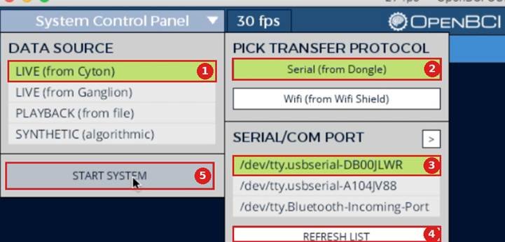
The System Control Panel, step by step. 1. Choose LIVE (from Cyton). 2. Choose Serial (from Dongle). 3. Pick the dongle’s port; on a Mac it starts with /dev/tty.usbserial, on Windows it is COM plus a number. Ignore Bluetooth ports. 4. Click Refresh List only if the port is missing. 5. Click START SYSTEM.
What it means
The System Control Panel, the first screen you see, offers four data sources:
| Data source | What it does | When to use it |
| LIVE (from Cyton) | Streams from a Cyton or Cyton + Daisy board | Real recordings |
| LIVE (from Ganglion) | Streams from the smaller 4-channel Ganglion | Real recordings on a Ganglion |
| PLAYBACK (from file) | Replays a recording you made earlier | Reviewing data; demos without hardware |
| SYNTHETIC (algorithmic) | Generates fake but realistic signals | Learning the software before the kit arrives |
Once data is streaming, the GUI saves everything automatically to a folder on your computer (Documents → OpenBCI_GUI → Recordings), with each session named by date and time. The files are plain text that opens in Excel, Python or MATLAB.
Why it is useful
- No waiting on a programmer. A student can collect a first dataset the same afternoon the kit arrives.
- Practice without hardware. Synthetic mode lets you learn every menu and widget before you have a board, or while someone else is using it.
- A safety net for demos. Record a clean session in advance. If the live setup fails on the day, switch to Playback and the demo continues with real data.
- Revisiting sessions. Playback lets you replay a recording and look again at a moment you missed live, with all the widgets working.
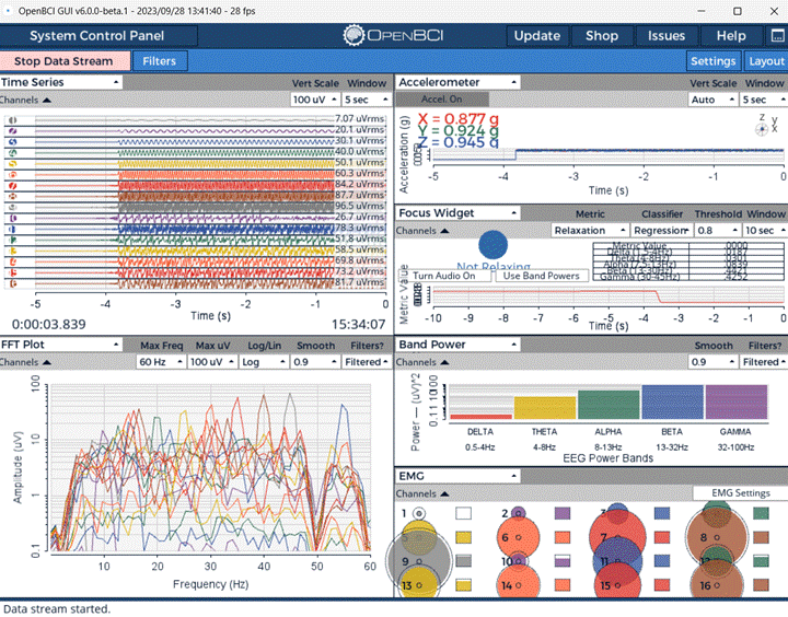
The GUI with six widgets running at once on a 16-channel stream: Time Series and FFT Plot on the left; Accelerometer, Focus, Band Power and EMG on the right. Every widget works the same whether the data is live, replayed from a file, or synthetic.
How to do it
- Plug in the dongle first, then switch the Cyton to PC.
- In the System Control Panel, choose LIVE (from Cyton), then Serial (from Dongle), then the dongle’s port.
- If you have a Daisy, set the channel count to 16. It defaults to 8, and channels 9 to 16 will not appear otherwise.
- Click START SYSTEM, then Start Data Stream.
- When finished, click Stop Data Stream. Your file is already saved.
Watch out: write a short note for every session: who, when, what they did, and anything odd (a sneeze, a loose electrode). Automatic file names record the time, not the context, and a month later you will not remember which file was which.
3. Working across macOS, Windows and Linux
The GUI runs as a standalone application on all three major operating systems, so it fits whatever computers your lab, classroom or home already has.
Why it is useful
- Mixed labs. Research groups rarely standardize on one system. A student on a Mac and a supervisor on Windows can run the same software, follow the same guide and open the same files.
- Old hardware gets a second life. A spare Linux laptop makes a perfectly good dedicated recording machine.
- Shared files. A recording made on one system opens on any other, which matters when data moves between collaborators.
How to do it
Download the version for your system from OpenBCI’s website and follow its install guide. Two system-specific details trip people up:
| Issue | Systems affected | What to do |
| The computer does not see the dongle | Some Windows and Mac setups | Install the FTDI VCP driver that OpenBCI’s install guide links to |
| Data arrives in choppy bursts, about once a second | Windows and some older Macs | A driver setting called FTDI latency is too high; OpenBCI’s FTDI Driver Fix guide lowers it |
| The dongle’s port name looks unfamiliar | All | It is named COM plus a number on Windows, and starts with /dev/tty on Mac and Linux |
Watch out: if several people use the kit on different computers, test the full setup on each machine before the day it matters. A driver problem discovered during a live session is far more stressful than one discovered the week before.
4. Filtering data in real time
Filters clean the signal as it arrives, removing the parts you do not want so the brain activity underneath becomes visible.
What it means
Raw EEG mixes brain activity with several kinds of unwanted signal: slow drift from sweat and shifting electrodes, hum from the building’s electrical wiring, and fast noise from muscles and electronics. Click Filters at the top of the GUI to apply two main kinds of filter:
- Bandpass filter: keeps only a range of frequencies and throws away everything outside it. A range of about 1 to 50 Hz keeps the main brain rhythms and removes slow drift and very fast noise.
- Notch filter: removes one narrow frequency, the electrical hum from wall power. Set it to 60 Hz in North America, and 50 Hz in Europe, Africa and most of Asia.
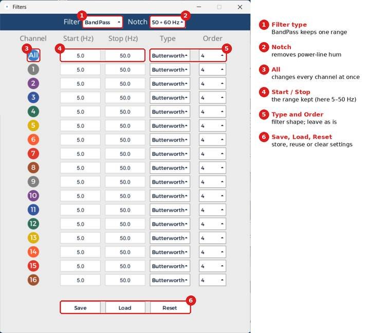
The Filters window. Here it keeps 5 to 50 Hz on every channel, and the notch is set to “50 + 60 Hz”, which removes power-line hum anywhere in the world. Change the All row to update every channel at once. For demos that include eye movements, lower Start to 1 Hz so those slow signals stay visible.
BandPass or BandStop? The filter type menu offers two opposite choices. BandPass keeps the range between Start and Stop and removes everything else, like a bouncer who only lets in people aged 5 to 50. BandStop does the reverse: it removes that range and keeps everything outside it, which would throw away the brain rhythms you care about. For EEG, leave it on BandPass. The notch filter is already a very narrow BandStop aimed at power-line hum, so you rarely need to choose BandStop yourself.

Why it is useful
- A readable live view. Without filters, slow drift and hum can swamp the screen and hide everything else.
- Trustworthy live judgments. Decisions you make during a session, such as “this electrode needs more gel”, depend on a clean view.
- Better demos. A filtered signal shows blinks, jaw clenches and alpha rhythms clearly to an audience.
How to do it
- Click Filters.
- Set the notch to your country’s power frequency.
- Choose a bandpass range. Use 1 to 50 Hz for general EEG; widen the top end if you are studying muscle activity, which reaches higher frequencies.
- In the FFT plot, check that the Filtered option is on, and compare it with Unfiltered to see what the filters removed.
Watch out: the GUI’s filters change what you see, but the saved recording still holds the raw, unfiltered data. That is a good thing: it means you can choose your final filters carefully during analysis. Just remember to apply them again in Python or MATLAB, rather than assuming the file is already clean.
5. Running your own experiments and replicating classic research
With a consumer kit and the GUI, you can test your own ideas and repeat well-known findings from decades of brain research, at home or in a teaching lab.
Why it is useful
- Learning by doing. Repeating a famous finding yourself teaches more about EEG than any textbook chapter.
- Checking your setup. If a classic effect appears, your equipment and method are working. If it does not, something is wrong before you run anything new.
- Cheap pilot studies. Before applying for funding or ethics approval for a big study, a small pilot shows whether the idea is feasible.
- Teaching. Students can run real experiments in a single lab session.
Classic experiments to try, easiest first
| Experiment | What you do | What you should see | Difficulty |
| Blinks and jaw clenches | Blink, look left and right, clench your teeth | Large spikes on forehead electrodes; fuzzy bursts near the temples | Very easy |
| Eyes-closed alpha | Alternate 10 seconds eyes open, 10 seconds closed | A bump around 10 Hz on the back-of-head electrodes when eyes close | Easy |
| Flicker response (SSVEP) | Look at a light or screen flashing at a steady rate | A peak in the FFT at exactly the flicker frequency | Moderate |
| Imagined movement | Imagine squeezing your left or right hand | A drop in the 8 to 12 Hz rhythm over the opposite side of the head (electrodes C3 and C4) | Harder |
| Surprise response (P300) | Watch a stream of images where one kind appears rarely | A brain response about 0.3 seconds after each rare image, visible only after averaging many trials | Harder |
Which electrodes to use. Each experiment shows up best at particular spots on the head. The channel number in the GUI depends on which board pin you plug each electrode into.
| Experiment | Best electrodes | Where on the head |
| Blinks and eyebrow raises | Fp1, Fp2 | Forehead, above the eyebrows |
| Looking left and right; jaw clenches | F7, F8 (also T3, T4 for jaw) | Temples, beside the eyes |
| Eyes-closed alpha | O1, O2 (also P3, Pz, P4) | Back of the head |
| Flicker response (SSVEP) | O1, O2 | Back of the head, over the vision area |
| Imagined movement | C3, C4, Cz | Top of the head; C3 reflects the right hand, C4 the left |
| Surprise response (P300) | Pz, Cz (also P3, P4) | Top and upper back of the head |
For example, with Fp1, Fp2, F7, F8, O1 and O2 plugged into Cyton pins N1P to N6P in that order, they appear as channels 1 to 6.
The first two need nothing but the GUI. The last two depend on knowing exactly when each event happened, which brings in markers.
Markers: the key to real experiments
A marker is a label stamped into the recording at the instant something happens: “image shown”, “warning appeared”, “participant pressed a key”. Without markers, you have a long recording and no way to line it up with your task. With them, you can cut out the moment after each event and compare conditions. The GUI includes a Marker widget for adding them, and experiment software such as PsychoPy can send them automatically (see use case 7).
How to design a good experiment
- Ask one clear question, such as “Does alpha rise when eyes close?”
- Record a baseline: a minute of sitting quietly, so you know each person’s normal activity.
- Repeat each condition many times. One eyes-closed period proves little; ten are convincing.
- Keep everything else the same: room, instructions, time of day.
- Mark every event so you can line up the data with what happened.
- Get ethics approval before testing anyone other than yourself for research purposes. Universities require it for any study with participants.
Worked example: designing the eyes-closed alpha test
Here is the whole process for one simple experiment, from question to answer. It takes about 30 minutes with one person.
1. Write the question and your prediction. Question: does alpha rise when the eyes close? Prediction: power in the 8 to 12 Hz range, measured at the back of the head, will be higher during eyes-closed periods than eyes-open ones.
2. Choose the electrodes. Use O1 and O2 at the back of the head, where alpha is strongest, plus REF and GND, which every recording needs. Optionally add Fp1 on the forehead: alpha should barely change there, which gives you a useful comparison.
3. Set up and check the signal. Fit the cap, add gel, and wait until O1 and O2 read Not Railed with small µVrms values. Set the notch filter to 60 Hz (50 Hz outside North America) and the bandpass to 1 to 50 Hz.
4. Arrange the screen. Show Time Series, FFT Plot, Band Power and the Marker widget. Agree a marker code: 1 = eyes closed, 2 = eyes open.
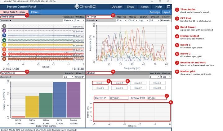
The screen arranged for the alpha test. The Time Series (1) checks each channel, the FFT Plot (2) shows the 10 Hz alpha bump, and Band Power (3) shows the alpha bar rising when the eyes close. In the Marker widget (4), click Insert 1 (5) when the eyes close and Insert 2 (6) when they open; each marker appears on the plot below (8). The Receive IP and Port (7) let other software, such as PsychoPy, send markers automatically.
5. Plan the timing. Use alternating blocks of 20 seconds, 10 eyes-closed and 10 eyes-open, about 7 minutes in total. Repeating the switch many times is what makes the result convincing. Use a phone timer, or have a helper say “close” and “open” at each change.
6. Give clear instructions. Ask the participant to sit still, keep their jaw and face relaxed, and avoid talking. With eyes open, they look at one fixed spot. Muscle tension and movement create noise that can hide alpha.
7. Run it. Start the data stream and record one minute of quiet sitting with eyes open as a baseline. Then begin the blocks, clicking marker 1 each time the eyes close and 2 each time they open. Write down anything unusual, such as a cough, a blink burst or someone entering the room.
8. Analyse. Open the saved file in Python or MATLAB. Use the markers to split the recording into eyes-closed and eyes-open segments, measure the 8 to 12 Hz power in each, and compare the averages for O1 and O2.
9. Interpret honestly. If eyes-closed alpha is clearly higher at O1 and O2, but not at Fp1, your setup records real brain activity and the prediction is supported. If there is no difference, check electrode contact at the back of the head before concluding anything: hair often keeps O1 and O2 from touching the scalp properly.
The same nine steps fit almost any EEG experiment. Change the question, the electrodes and the task, and the structure stays the same.
Using markers during the alpha test, step by step
What a marker code is. Decide before you start what each marker number means, write it down, and make sure anyone helping uses the same code. Here, 1 = eyes just closed and 2 = eyes just opened. A marker only stores a number, so the code is what gives it meaning later.
Where to sit. Sit at the computer beside or slightly behind the participant, with the screen turned away from them; watching their own brainwaves distracts people and makes them move. Keep still and quiet yourself, and do not touch the cap or cables while recording.
The sequence.
- Start the data stream and record one minute of quiet sitting with eyes open as a baseline.
- Say “close” and click Insert 1 at the same moment.
- Wait 20 seconds.
- Say “open” and click Insert 2 at the same moment.
- Wait 20 seconds.
- Repeat steps 2 to 5 until you have done 10 rounds, about 7 minutes in all.
Click as you speak, not afterwards, so each marker matches the moment the eyes change. If speaking and clicking at once feels awkward, a helper can give the cues while you click, or a phone timer can beep at each change. Keep each eyes-closed period between about 10 and 30 seconds: shorter gives too little data, and longer risks drowsiness, which changes the brain’s rhythms. For a quick live demo, a single 10-second eyes-closed period is enough to show the effect.
What each click does. Think of a marker as a sticky note on a video timeline. The recording is saved like a long spreadsheet: one row for each tiny slice of time, hundreds per second, with a column for each electrode and one for markers. The marker column normally reads 0. When you click Insert 1, the row for that exact moment gets a 1 instead. Later, you search the file for the 1s and 2s to find exactly when the eyes closed and opened.
How to tell it worked. In the Marker widget’s graph, the line normally lies flat along 0. Each click makes a short spike at the right-hand edge, which is “now”: height 1 for Insert 1, height 2 for Insert 2. The spike drifts left and disappears after 5 seconds, the width of the window.
Receive IP and Port. These fields let another program on the computer send markers for you. That matters when software shows pictures and needs perfect timing. For the alpha test, you can ignore them and click by hand.
Practise first in Synthetic mode. You can rehearse everything without the cap: set up the layout, click the marker buttons, watch the spikes appear, then open the saved file and find the 1s and 2s. What you will not see is the alpha effect itself. Synthetic data is generated by the computer and does not react to anyone’s eyes, so the alpha bump only appears with the real cap on a real person.
After the recording: what next
- Stop and save. Click Stop Data Stream. The recording saves automatically to Documents → OpenBCI_GUI → Recordings.
- Write a quick note. Record who took part, the date and time, and anything unusual, such as coughs, movement or a loose electrode.
- Check it without code. Replay the file in Playback mode and watch the FFT Plot and Band Power. Alpha should rise after each marker 1 and drop after each marker 2.
- Analyse it properly. Open the file in Python or MATLAB. Use the 1s and 2s in the marker column to cut out the eyes-closed and eyes-open stretches, measure the 8 to 12 Hz power at O1 and O2 in each, and compare the averages, as in step 8 above.
Watch out: vague stimuli give vague results. Playing music or showing a surprising video and “seeing what happens” rarely produces a clear pattern, and any change is often muscle movement rather than brain activity. Start with the classic, well-understood effects above.
6. Skipping the setup headaches
Getting data out of an OpenBCI board with your own code means installing a programming language, the right libraries and drivers, then writing connection code. The GUI packages all of that into one download.
What it means
Under the hood, the GUI uses BrainFlow, a free library that knows how to talk to OpenBCI boards and many others. Without the GUI, a typical do-it-yourself route looks like this:
- Install Python.
- Install BrainFlow and other packages, and fix any version clashes.
- Find the dongle’s port name.
- Write a script that connects, starts the stream, reads data and saves it.
- Write more code to plot it, so you can check whether it is working at all.
Each step is a place where beginners get stuck. The GUI replaces all five with “download, open, click Start”.
Why it is useful
- Non-programmers can use EEG. Students in psychology, business, education or the arts can collect data without learning to code first.
- Fewer moving parts. When something goes wrong, there are far fewer places to look.
- A known-good reference. If your own script misbehaves, checking the same board in the GUI tells you instantly whether the problem is the hardware or your code.
How to do it
Install the GUI and open it in Synthetic mode first. If fake signals appear, the software is installed correctly, and any later problem is about the board, dongle or drivers rather than the installation.
| First-run problem | Likely cause | Fix |
| Dongle’s port not listed | Missing driver, or dongle switch on RESET | Install the FTDI driver; set the switch to GPIO6; click Refresh List |
| Connection fails | Board off or started in the wrong order | Plug in the dongle first, then switch the board to PC; restart the system |
| No radio channel shown | Board and dongle on different channels | Use AUTOSCAN under Radio Configuration in the System Control Panel |
Watch out: the GUI and your own script cannot both connect to the board at the same time, because only one program can use the dongle at once. Close the GUI’s session before running a script, or use the GUI’s streaming features instead (next section).
7. Streaming data into MATLAB, Python and other apps
The GUI can pass the live data on to other programs as it arrives, so you can analyse it, react to it or build something with it, while still using the GUI to watch signal quality.
What it means
This happens through the Networking widget. Set any panel to Networking, choose a method and what to send, and click Start. The data travels on to other programs on the same computer or the local network.
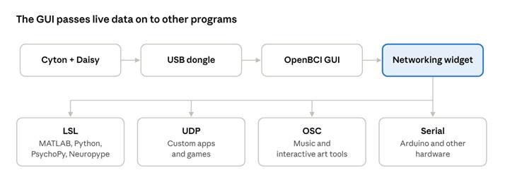
data path from board to other programs · 4 streaming methods
The four methods differ in what they connect to:
| Method | Plain-language description | Typical use |
| LSL (Lab Streaming Layer) | A research standard for sharing time-stamped data between programs | MATLAB, Python, PsychoPy, Neuropype; syncing EEG with experiment events |
| UDP | A simple, fast way to send data over a network | Custom programs and games |
| OSC | A messaging format popular with creative software | Music, sound and interactive art projects |
| Serial | A wired connection to small hardware | Driving an Arduino, lights or motors |
You also choose what to send: the raw time series, the FFT, band power, or other processed values. Sending band power, for example, gives a program five simple numbers to react to, rather than a fast stream of raw samples.
Why it is useful
- Real analysis tools. MATLAB and Python offer far more analysis than the GUI. Streaming lets you process data live with them.
- Proper experiments. Experiment software such as PsychoPy shows stimuli and records responses. Through LSL, its event markers and the EEG share one clock, so you know exactly which brain activity followed which stimulus. This is how serious research setups work.
- Neurofeedback and interactive projects. A program can change music, colours or a game based on, say, the wearer’s alpha level.
- Combining signals. LSL can bring EEG together with other devices, such as heart rate or skin conductance sensors, on one timeline.
How to do it
- Start the session and data stream as usual.
- Switch one panel to Networking.
- Choose LSL for research use, and select the data type to send, such as the time series.
- Click Start in the widget.
- In MATLAB or Python, use an LSL library (for example liblsl-Matlab or pylsl) to find the stream by name and read from it.
Watch out: the GUI’s recording and your streamed copy are separate. If your analysis program crashes, the GUI’s file is still safe, so keep the GUI recording running as a backup.
Putting it together: one project, all seven use cases
The seven use cases are not separate features you pick between. A real project uses all of them in sequence. Here is how a small research pilot might run, asking: do people stop paying attention to an on-screen warning when they see it again and again?
- Practise without hardware (use cases 2 and 6). Before the kit is free, install the GUI and explore it in Synthetic mode. Confirm the installation works and learn the widgets.
- Set up on the lab computer (use case 3). Install the drivers on the machine you will actually use, and test the dongle connection the week before.
- Check signal quality (use case 1). With the cap on, use the Time Series until every channel you need reads Not Railed with small values. Do the eyes-closed alpha test to confirm real brain signals are coming through.
- Clean the live view (use case 4). Set the notch to 60 Hz and a 1 to 50 Hz bandpass, so you can monitor quality during the session.
- Run the task with markers (use cases 5 and 7). PsychoPy shows the warning many times while sending a marker over LSL each time it appears. The GUI streams the EEG over LSL, so both share one clock.
- Record everything (use case 2). The GUI saves the raw recording automatically as a backup, while your experiment software logs responses.
- Analyse afterwards. In Python or MATLAB, apply your chosen filters, cut out the second after each warning, and compare the brain’s response to the first showings with the later ones.
None of these steps requires custom hardware or expensive software. The GUI does the connecting, checking and recording, and hands off to specialist tools only where they add something.
Choosing the right tool for your goal
| Your goal | Start with |
| See whether the equipment works | Time Series and FFT widgets |
| Run a live demo or teach a class | Time Series, EMG and Band Power side by side; a backup recording for Playback |
| Collect data quickly with no coding | The GUI’s automatic recording |
| Learn before the hardware arrives | Synthetic mode |
| Run a proper experiment with stimuli | PsychoPy (or similar) plus LSL markers, with the GUI recording as backup |
| Analyse data in depth | Python or MATLAB, on the saved file or a live LSL stream |
| Build an interactive or neurofeedback project | The Networking widget, sending band power over UDP or OSC |
| Write fully automated pipelines | BrainFlow in your own code, without the GUI |
Know the limits
- It is not a medical device. OpenBCI equipment is for research, education and exploration, not for diagnosing or treating anyone.
- Consumer EEG is noisy. Clear, repeatable effects (blinks, alpha, flicker responses) work well. Subtle effects need careful design, many trials and good electrode contact.
- The GUI is for exploring and recording, not final analysis. Treat its widgets as a window onto the data and its files as raw material. Serious analysis happens afterwards, in dedicated tools.
- People need protecting. Any study with participants, beyond trying it on yourself, needs approval from a research ethics board first.
Final thought
The OpenBCI GUI lowers the barrier to brain research further than almost any tool before it. In one afternoon, a beginner can see their own brainwaves, record them, clean them and send them to a program of their own. The equipment will not make anyone a neuroscientist overnight, but used carefully, with good contact, clear questions and honest analysis, it makes real research possible on a student’s budget.